Cycles of polynomial maps
This page is about an algorithm for computing the exact
n-cycles of some polynomials maps.
Introduction
Consider a one-dimensional map,
x
→
f (x),
where f(x) is some polynomial function.
If we iterate the map many time, we would have an iteration sequence:
xk+1
= f (xk).
Occasionally, this sequence would go back to some previous value after a few iterations,
and afterwards, it simply repeats itself.
This is what we call a cycle.
The mathematical problem we wish to figure out is that when does such a cycle happen.
Cycles and fixed points
An n-cycle is a sequence
x0,
x1,
...
xn,
such that
xn
= x0.
Here, n has to be the
smallest positive integer that satisfies the relation.
After the first cycle, the pattern would repeat itself, and we would have
x n+k
= xk
for k.
Particularly, a 1-cycle
is called a fixed point, that is, the solution of
f (x0)
= x0.
Any cycle point
xk
in the n-cycle of f
is also be a fixed point of the iterated map
fn,
(which is called the nth iterate of f) for
xn+k
= fn(xk )
= xk.
However, a fixed point of
fn
(n > 1)
is not necessarily a n-cycle point.
For example, a fixed point of
f
is also a fixed point of its nth iterate,
but is not qualified as a ncycle point.
Stable cycles
A cycle can be stable or unstable.
In a stable cycle,
a small deviation from the exact cycle point
x0
gets reduced in magnitude after n iterations,
such that xn becomes closer to the exact cycle point
than x0.
In other words, a stable cycle is attractive in the neighborhood of its cycle points.
A stable cycle is generally more meaningful than an unstable one.
If we start the iteration from a random
x0
it will be converged only to a stable cycle.
We further note that if
xk
are complex numbers,
a cycle always exists, for we can always find complex roots
of the algebraic equation
fn(x) = x.
Statement of the problem
Now let us say the map
f
depends on a parameter
r.
For example, in the logistic map,
f (x)
≡ r x (1 − x).
Both the cycle points and the cycle stability of a cycle depend on the parameter
r.
The problem we are trying to tackle here is
to determine the
r values
that allow stable n-cycles.
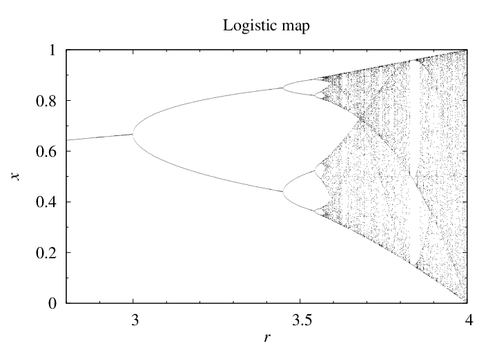
Bifurcation diagram
Stable cycles can be visualized in a bifurcation diagram
as shown below (for the logistic map).
Starting from a random x0 (0.1 here),
the final xk points
after a large number of iterations are plotted
against the value of the parameter r.
Obviously, all xk points shown in the plot
belong to a stable or attractive cycle.
Onset and bifurcation points
Our purpose is to determine the r values at which
stable n-cycles exist.
As we usually are interested in real
r
and
xk,
the r
values for stable cycles are arranged as
windows on the real axis.
For example, as shown in the above figure (logistic map),
the stable 2-cycle exists in the window
(3, 1 + √6) = (3, 3.449...).
We shall call the two bounds as the
onset and bifurcation points
of the cycle.
For a polynomial map,
the r values at the onset and bifurcation points
are algebraic numbers,
i.e., they are zeros of some polynomials of integral coefficients.
Our problem is, therefore, to find one polynomial
that encompasses all onset r values as the zeros,
and the other polynomial for all bifurcation r values.
Derivative condition
The onset and bifurcation points of the n-cycle
can be determined from the derivative of the composite map
[ f n(x) ]′
= [ f (⋯( f (x)⋯) ]′
.
Since a stable cycle must reduce the magnitude of
x
after
n
successive iterations,
the magnitude of this derivative must be 1.0 at the two critical points.
More precisely, +1 and −1 are assigned to
the onset and bifurcation points, respectively.
Thus by the chain rule, we have
f ′(x1)
⋯
f ′(xn)
= ±1,
at the onset (+1) and bifurcation (−1) points.
The
n
equations,
xk+1
= f (xk)
(with
xn = x0),
along with the derivative condition,
furnish
n + 1 equations.
Thus, we can eliminate the n variables
xk
and obtain the desired equation of
r.
Individual maps
Individual maps has separate pages. The onset and bifurcation polynomials can be found there.
- The logistic map
- The cubic map
- The Hénon map
Programs
For convenience, we list a few main programs here.
| Program | Description |
|---|---|
| log.ma | A Mathematica script for the cycle polynomials of the logistic map |
| cub.ma | A Mathematica script for the cycle polynomials of the cubic map. |
| hen.ma | A Mathematica script for the cycle polynomials of the Hénon map. |
| lsfit.ma | A specialized Mathematica script that interpolates a polynomial from a list of values, generated by log.ma or cub.ma after a parallel or unfinished run see here. |
| mkinterp.py | A Python script that generates a specialized Mathematica script, which interpolates a polynomial from a list of values. For logistic and cubic map, use the faster lsfit.ma in the above instead. Reserved for the Hénon map. |
| mknsolv.py | A Python script that generates a specialized Mathematica script, which numerically solves zeros of the polynomial r-cycles (the output of lsfit.ma.) |
A note on the Mathematica scripts (.ma files)
The “.ma” file,
listed here, are plain-text Mathematica scripts.
The extension
“.ma”
is arbitrary, it can also be
“.txt”.
Unlike the Mathematica notebooks
(.nb files),
they do not contain formatting information
and can be edited by any text editor (e.g.,
Notepad,
Vim,
or
Emacs)
instead of the default Mathematica GUI editor.
To run such a script
(say myprog.ma), type in the command-line
math < myprog.ma argument1 argument2 ...
Here,
math
(or math.exe in Windows)
is the file name of Mathematica's main command-line driver,
which should be installed under same directory
as the GUI interface
mathematica
(or Mathematica.exe in Windows).
If this directory is not added in the environment variable
PATH,
the full path to
math
should be used in the above command.
References
General
- Robert M. May, Simple mathematical models with very complicated dynamics, Nature 261 (1976) 459-467.
- Steven H. Strogatz, Nonlinear Dynamics And Chaos: With Applications To Physics, Biology, Chemistry, And Engineering" Westview Press, 2001.
- Bailin Hao, Elementary Symbolic Dynamics and Chaos in Dissipative Systems, World Scientific, 1989. See the ESD page for more about the book.
Primary reference
- Cheng Zhang, Cycles of the logistic map, International Journal of Bifurcation and Chaos 24 (2014) 1450005; also, an earlier preprint: arXiv:1204.0546, 2012.
Last updated on April 2nd, 2014.