Cycles of the logistic map
Introduction
Simplified logistic map
If we further allow complex R and xk , then we may set d = exp(i θ) with θ running continuously from 0 to 2π. Doing so allows us to obtain continuous curves of R (instead of just two points) on the complex plane, which enclose regions of R that contain complex stable cycles.
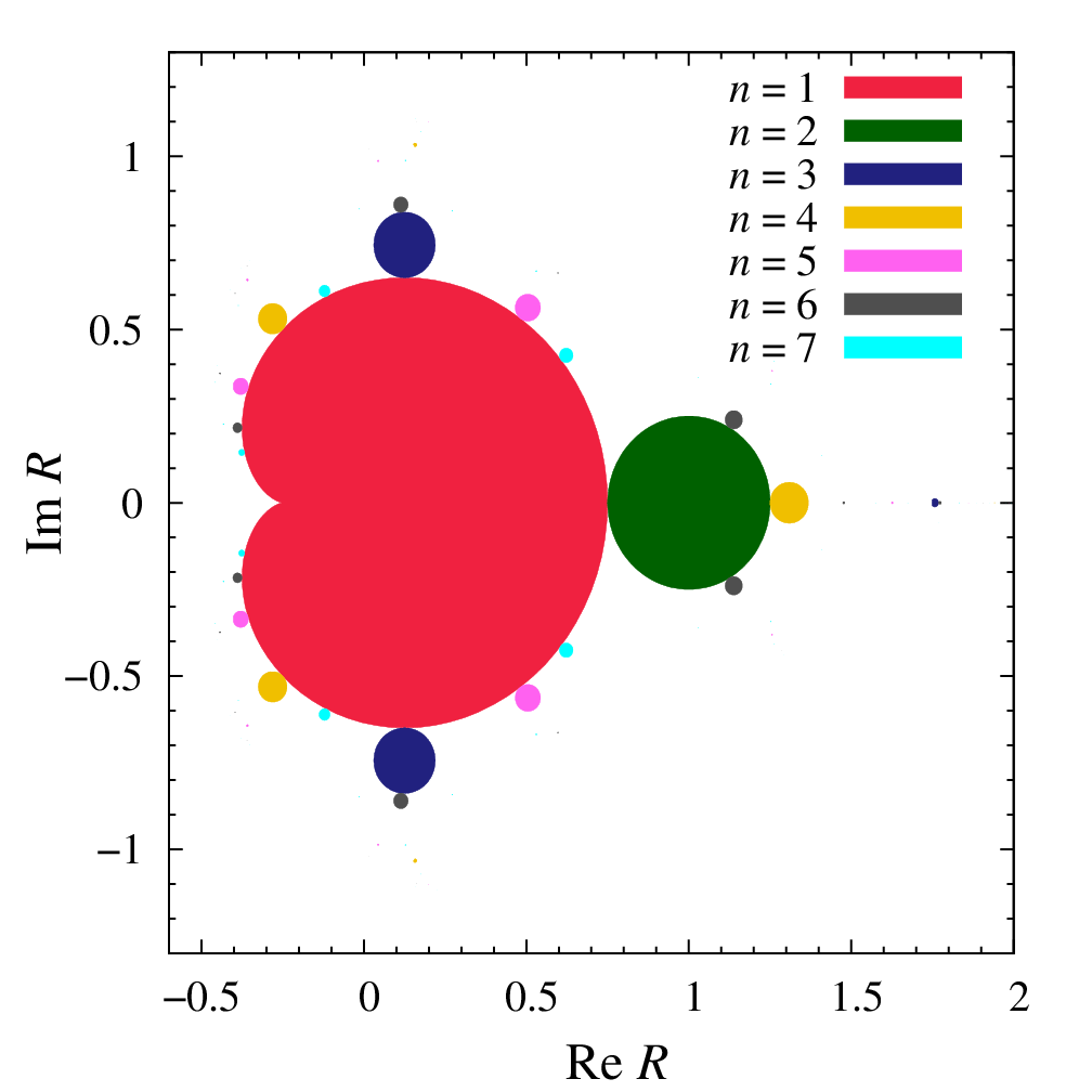
The resulting figure is in fact the inverted Mandelbrot set. With zk = −xk and c = −R. The modified logistic map becomes the quadratic map zk+1 = zk2 + c that is used to generate the Mandelbrot set.
3-cycle
While the 1-cycle (fixed point, −1/4 < R ≤ 3/4 or 1 < r ≤ 3) and 2-cycle (3/4 < R ≤ 7/4 or 3 < r ≤ 1+√6) are generally easy to obtain (Strogatz), the 3-cycle (n = 3) is not quite obvious. The onset values R = 7/4 or r = 1 + √8 of the 3-cycle is nonetheless quite simple, and hence has been derived in several papers by different methods (see the References).
A brief and self-contained derivation of the onset and bifurcation points of the real 3-cycle is presented in the note (PDF, HTML).
As a side note, the existence of the 3-cycle in a general map is quite important, as it implies the existence of cycles of all other lengths, thus chaos (Sharkovskii and Li & Yorke).
n-cycles
n-cycle data
| n | Onset | Bifurcation | General |
|---|---|---|---|
| 1 | Poly., PNG and r values | Poly., PNG and r values | R-X |
| 2 | Poly., PNG and r values | Poly., PNG and r values | R-X |
| 3 | Poly., PNG and r values | Poly., PNG and r values | R-X |
| 4 | Poly., PNG and r values | Poly., PNG and r values | R-X |
| 5 | Poly., PNG and r values | Poly., PNG and r values | R-X |
| 6 | Poly., PNG and r values | Poly., PNG and r values | R-X |
| 7 | Poly., PNG and r values | Poly., PNG and r values | R-X |
| 8 | Poly., PNG and r values | Poly., PNG and r values | R-X |
| 9 | Poly., PNG and r values | Poly., PNG and r values | R-X |
| 10 | Poly., PNG and r values | Poly., PNG and r values | R-X |
| 11 | Poly., PNG and r values | Poly., PNG and r values | R-X |
| 12 | Poly., PNG and r values | Poly., PNG and r values | |
| 13 | Poly., PNG and r values | Poly., PNG and r values | |
| 14 | Poly., PNG and r values | Poly., PNG and r values |
Programs
| Program | Description |
|---|---|
| log.ma | A self-contained Mathematica script that computes the onset, bifurcation
and general boundary polynomials of R
for the n-cycles.
For the onset polynomial of the 9-cycles, type
math < log.ma 9 a
The output would be
T9a.txt
and
r9a.txt.
For the bifurcation polynomial of the 8-cycles, type
math < log.ma 8 b
The output would be
T8b.txt.
For the general boundary polynomial of the 7-cycles, type
math < log.ma 7 X
The output would be
RX7.txt.
A variant can be accessed through
“Y”
(faster for longer cycles)
instead of
“X”.
For the tupling (which is a generalization of period-doubling in the complex plane) polynomial of the intersection of the 5-cycles and 35-cycles, type
math < log.ma 5 x 35
The output would be
T5x35.txt.
|
| lsfit.ma |
A specialized Mathematica script
that interpolates a polynomial
from a list of values.
This script is intended for parallelization, which should be invoked
only if the computing time is limited.
For small n,
a simple call to log.ma will save
much trouble.
To parallelize the calculation of the bifurcation polynomial for the 8-cycles, we can compute the first 60 R values (the degree in R is 120, and R runs from −60/4 to −1/4)
math < log.ma 8 b -60 0
This will create a file called
ls8b.txt.
On another computer node, we do it again for the other half
(such that R runs from 0/4 to 60/4)
math < log.ma 8 b 0 61
This will create another
ls8b.txt.
(If the two commands are run under the same directory,
but at different times, the latter will simply append new values
to the existing ls8b.txt.)
We should now combine the contents in the two files.
We now type
math < lsfit.ma ls8b.txt 2 1
The interpolated polynomial from the values in
ls8b.txt
are then saved to
fit.txt.
Here, the second number 2 is the method index. If it is 0, it means to use Mathematica's built-in function InterpolatingPolynomial[]. This built-in function is quite fast. But it may fail sometimes. If it is 1, it will compute the interpolating polynomial from top (the leading coefficients) to bottom. Method 1 is robust, but very slow. If it is 2, it will compute the interpolating polynomial from bottom to top. Method 2 is quite fast, and is therefore recommended. The last number 1 is the verbosity level. Using method 2, the script also checks for potential corruptions in the list values (which can happen!) that prevents the final result to be an integral polynomial. |
|
|
To parallelize the calculation of the bifurcation polynomial for the 8-cycles, we can compute the first 60 R values (the degree in R is 120, and R runs from −60 to −1)
math < log.ma 8 b -60 0
This will create a file called
ls8b.txt.
On another computer node, we do it again for the other half
(such that R runs from 0 to 60)
math < log.ma 8 b 0 61
This will create another
ls8b.txt.
(If the two commands are run under the same directory,
but at different times, the latter will simply append data
to the existing ls8b.txt.)
We should now combine the contents in the two files.
We now type
python mkinterp.py ls8b.txt
which will generate a Mathematica script
fit.ma.
Finally, the interpolated polynomial from the values in
ls8b.txt
can be obtained from
math < fit.ma
The result is saved to
fit.txt.
|
| mknsolv.py | A Python script that generates a Mathematica script, which numerically solves the R values of the onset or bifurcation polynomial equations. |
| logres8b.magma | A
magma
script
that solves the bifurcation polynomial of 8-cycles by
computing the resultant.
The script works for the special case of the 8-cycle bifurcation point.
To use it, type
magma < logres8b.magma
Although it does not run as fast as the
log.ma,
it is much faster than
Mathematica’s
routine
Resultant[].
|
| mkgb.py | A Python script that generates a
magma
script,
which solves the boundary polynomial by
constructing a Gröbner basis
(which is the specialty of
magma).
For example, to compute the bifurcation polynomial of the 8-cycle for the simplified logistic map, type python mkgb.py 8 b > R8b.magma
Download
R8b.magma. Then call magma
magma < R8b.magma
To compute the onset polynomial of the original logistic map, type
python mkgb.py -r 8 a > r8a.magma
magma < r8a.magma The program does not run as fast as the log.ma, but it is much faster than Mathematica’s routine GroebnerBasis[]. |
References
Primary reference
- Cheng Zhang, Cycles of the logistic map, International Journal of Bifurcation and Chaos 24 (2014) 1450005; also, an earlier preprint: arXiv:1204.0546, 2012.
General information
- MathWorld
- Wikipedia
- Robert M. May, Simple mathematical models with very complicated dynamics, Nature 261 (1976) 459-467.
- Benoit B. Mandelbrot, Fractal aspects of the iteration of z → λ z (1 − z) for complex λ and z, Annals New York Academy of Sciences 357 (1980) 249-259.
- Steven H. Strogatz, Nonlinear Dynamics And Chaos: With Applications To Physics, Biology, Chemistry, And Engineering" Westview Press, 2001.
- Bailin Hao, Elementary Symbolic Dynamics and Chaos in Dissipative Systems, World Scientific, 1989.
Derivations of the n-cycle
- A. Brown, Equation for periodic solutions of a logistic difference equation, J. Austral. Math. Soc. Ser. B 23 (1981), 78-94.
- A. Brown, Solution of period seven for a Logistic difference equation, Bull. Austral. Math. Soc. 26 (1982), 263-284.
- John Stephenson, Formulae for cycles in the Mandelbrot set, Physica A 177 (1991) 416-420.
- John Stephenson and Douglas T. Ridgway, Formulae for cycles in the Mandelbrot set II, Physica A 190 (1992) 104-116.
- John Stephenson, Formulae for cycles in the Mandelbrot set III, Physica A 190 (1992) 117-129.
Derivations of the 3-cycle
- Partha Saha and Steven H. Strogatz, The birth of period three, Mathematics Magazine 68 (1995) 42-47.
- John Bechhoefer, The birth of period 3, revisited, Mathematics Magazine 69 (1996) 115-118.
- William B. Gordon, Period three trajectories of the logistic map, Mathematics Magazine 69 (1996) 118-120.
- Jacqueline Burm and Paul Fishback, Period-3 orbits via Sylvester’s theorem and resultants, Mathematics Magazine 74 (2001) 47-51.
- Cheng Zhang, Period three begins, Mathematics Magazine 83 (2010) 295-297; see also this note (PDF, HTML).
Period-3 implies chaos
- Alexander N. Sharkovskii (Oleksandr Mikolaiovich Sharkovsky), Co-existence of cycles of a continuous mapping of the line into itself, Ukrainian Matematicheskii Zhurnal, 16 (1964) 61-71.
- Tien-Yien Li and James A. Yorke, Period three implies chaos The American Mathematical Monthly 82 (1975) 985-992.
Number of roots
- Bailin Hao, Elementary Symbolic Dynamics and Chaos in Dissipative Systems, World Scientific, Singapore, 1989.
- Fa-geng Xie and Bai-lin Hao, Counting the number of periods in one-dimensional maps with multiple critical points, Physica A 202 (1994) 237-263.
- Bailin Hao, Number of periodic orbits in continuous maps of the interval—complete solution of the counting problem, Annals of Combinatorics 4 (2000) 339-346.
Last updated on April 2nd, 2014.